
Real vs Synthetic Training Data
I trained 13 YOLO26n detectors on the same 264 real game screenshots with different synthetic data and settings. This is the full training configuration, what each round changed, and the effect of the optimizer that Ultralytics selects automatically.
16 min read
I'm building an AI agent that plays Age of Empires II, a real-time strategy game. The agent has no access to the game's internal state. It only sees the screen, like a human player. On every turn, an object detector processes the screenshot and returns the visible objects with their class and position: villagers, animals, resources, buildings and military units. The agent plans its next action from that list.
This post is only about training that detector. It addresses a common question for small datasets: how much does synthetic training data help, and how is it best used?
The starting point
Labelling real screenshots is slow. A typical screenshot has 45 objects to box by hand, and I had 264 labelled screenshots. To fill the gap, the training set also had 2,400 synthetic images: sprites cut out of the game files and pasted onto generated backgrounds, with labels generated automatically. Two thirds of the training data was synthetic.
The goal of this work was to measure what those images are worth. Does the model get better with them, worse, or stay the same? And if they help, is there a better way to make or use them?
The first check was simple: compare the synthetic images with real ones. I measured the median box size of a few common objects:
Show the data
| Object | Synthetic | Real |
|---|---|---|
| villager | 27.8 px | 13.6 px |
| sheep | 32.5 px | 13.8 px |
| boar | 58.3 px | 18.1 px |
| house | 179 px | 66 px |
The synthetic objects were 2–3× bigger than the real ones. The generator drew sprites at full size on a 1280×720 canvas, while real screenshots are 3024 pixels wide and get shrunk to 42% before the model sees them. Scale augmentation (0.5–1.5×) can't close a gap that wide.
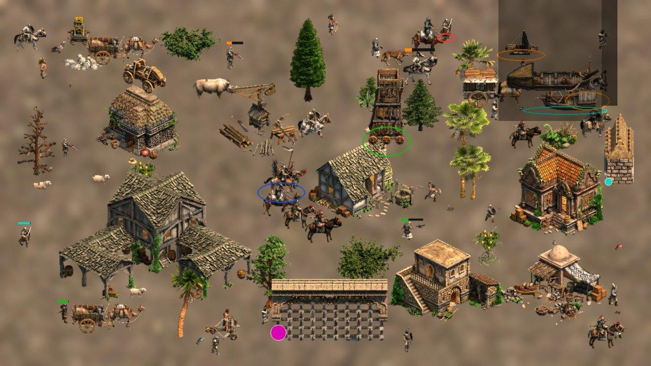
The synthetic data could still help despite the size mismatch, or it could teach the model incorrect object sizes. To measure this, I ran several training rounds with and without it and compared the results.
The detector
The model is YOLO26n from Ultralytics: a 2.6M-parameter detector, pretrained on COCO and fine-tuned on my data. It's the smallest YOLO26, because the agent needs a new detection every ~100 ms.
It learns 65 classes: trees, gold and stone mines, berry bushes, animals, buildings, villagers and military units. The screenshots are 3024×1672 and the model sees them at 1280 pixels wide, so a villager is ~14 pixels tall at the model input. This small object size is the main constraint behind the input resolution and several of the training choices below.
The real data is 264 screenshots with 11,842 boxes. Villagers, trees and houses make up half of the boxes. Some classes, like kings or trebuchets, have no real example at all and only exist in the synthetic data.
How I compared the runs
The validation set (8 screenshots) was too small to show meaningful differences between models: two earlier models scored F1 0.771 and 0.772, a gap within noise. For evaluation, I built a separate test set of 40 screenshots (1,248 hand-reviewed boxes) from 10 game sessions not used in any training run. The training script excludes those sessions to prevent leakage.
Each model is scored with the same confidence thresholds. A detection counts as correct if it overlaps the label with IoU ≥ 0.5. I report precision (the share of detections that are right), recall (the share of objects found) and F1, which combines the two.
Screenshots from the same game look alike, so I compare models per game session, with a permutation test. It gives a p-value: how likely a difference this big is if the two models were actually equal. On this test set, anything below ~0.02 F1 is noise.
The training setup
Every run in this post starts from this configuration. Each round changes one or two lines of it.
| Setting | Value | Why |
|---|---|---|
| Base model | yolo26n.pt (COCO weights) | small and fast enough for a detection every 100 ms |
| Input size | imgsz=1280 | objects are ~14 px at 1280; at 640 they'd be 7 |
| Epochs | 150 | |
| Early stopping | off (patience=0) | 8 validation screenshots can't decide when to stop |
| Saved model | the final epoch (last.pt) | same reason, no "best" checkpoint picked on 8 images |
| Batch size | 16, gradients accumulated to 64 | fits a 24 GB RTX 4090 at 1280 |
| Real images | each repeated 4× per epoch | 264 real against 2,400 synthetic; keeps real data at ~30% |
| Learning rate schedule | 3 warmup epochs, then linear decay to 1% | Ultralytics default |
| Weight decay | 0.0005 | Ultralytics default |
| Mixed precision | on | |
| Seed | 0, deterministic=True | |
| Optimizer | auto | Ultralytics default; see Round 3 |
Augmentation is close to the Ultralytics defaults, with two choices specific to a game:
| Augmentation | Value | Note |
|---|---|---|
| Mosaic | 1.0, off for the last 10 epochs | four images per training sample |
| Scale | 0.5 (random 0.5–1.5×) | |
| Horizontal flip | 0.5 | units face left and right |
| Vertical flip | 0.0 | fixed camera; objects never appear upside down |
| Rotation | ±10° | |
| Translate | 0.1 | |
| MixUp | 0.1 | |
| Colour (HSV) | 0.015 / 0.7 / 0.4 | player colours and fog change hue and brightness |
The hardware is one RTX 4090 (24 GB) per run, rented on RunPod. Images are cached in RAM to keep the GPU busy. An epoch takes 20–90 seconds depending on the dataset and model size, so a run takes 45 minutes to 4 hours. I ran up to three at once, one per pod.
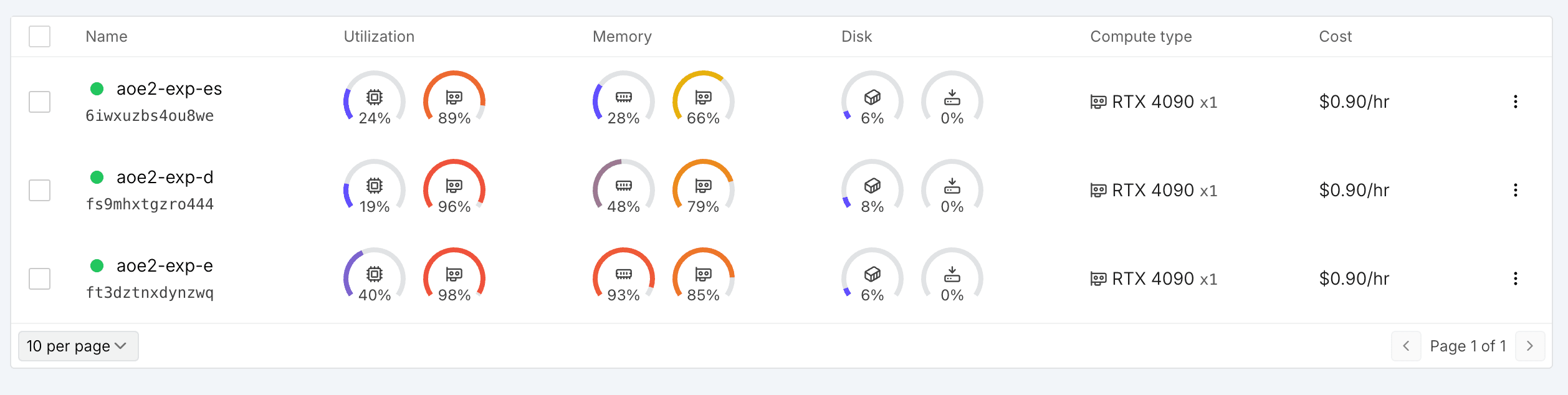
RAM limits differed between pods with the same GPU type: 31, 61 and 83 GB. Run E ran on the 31 GB pod with RAM caching and 16 data loader workers. At epoch 141 of 150, Ultralytics disables mosaic and rebuilds the data loader; worker memory briefly doubled and the pod terminated the run. Training can be resumed from the last checkpoint, with fewer workers if needed:
YOLO("runs/exp_e/weights/last.pt").train(resume=True, workers=8)Round 1: four ways to use synthetic data
The first round changes only the synthetic data. Everything else is the configuration above.
| Run | Real (×4) | Synthetic | Images per epoch | Training steps |
|---|---|---|---|---|
| Baseline | 1,056 | 2,400 old images (wrong size) | 3,456 | 32,400 |
| A | 1,056 | none | 1,056 | 9,900 |
| B | 1,056 | 1,000 composites (correct size), mixed in | 2,056 | 19,350 |
| C | 1,056 | 1,000 composites first (80 epochs, batch 8), then real only | 1,000, then 1,056 | 10,000 + 9,900 |
The composites address the size problem. Instead of drawing a background, the generator takes a real training screenshot and pastes sprites into it at the correct size. Real ground, fog and game interface are included automatically, and every object already in the screenshot has a label. Units go in as groups, never on black unexplored map and never over a labelled object. Trees and mines are not pasted, because real labels often put one box around a whole forest.
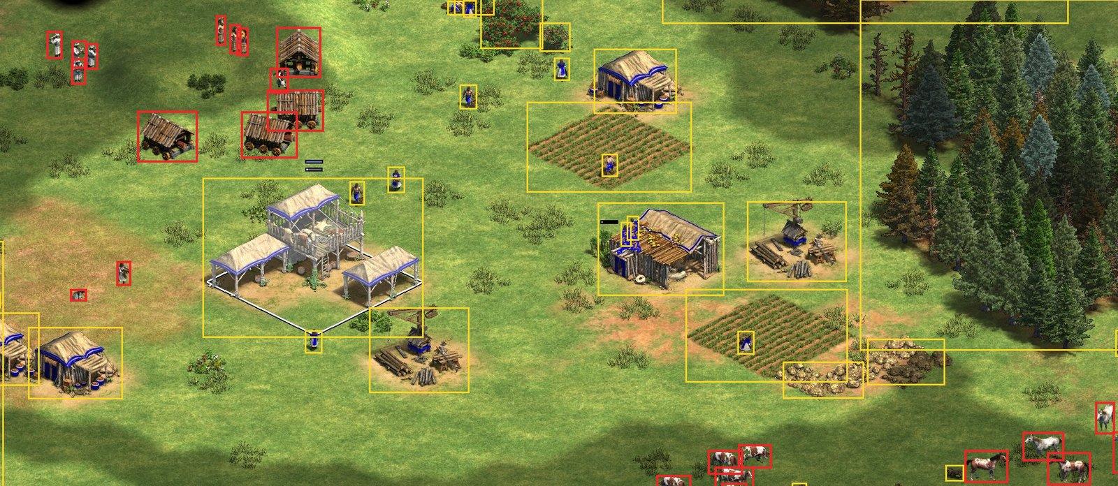
Run C used batch 8 for its pretraining phase. Composites are dense: a mosaic of four contains hundreds of boxes, and the label assigner ran out of GPU memory at batch 16.
The results:
Show the data
| Run | Precision | Recall | F1 |
|---|---|---|---|
| Baseline: real + old synthetic | 0.953 | 0.761 | 0.846 |
| A: real only | 0.925 | 0.690 | 0.790 |
| B: real + composites | 0.962 | 0.734 | 0.833 |
| C: composites, then real | 0.934 | 0.749 | 0.831 |
Removing the synthetic data reduced F1 by 0.056, the largest effect in this round. Composites improved on real-only training by ~0.04. Mixing (B) and pretraining (C) gave the same result, consistent with Burdorf et al.. Despite the correct scale, the composites did not outperform the old synthetic images.
Per-class results show where the difference comes from:
| Class | Test boxes | Baseline | A | B | C |
|---|---|---|---|---|---|
| sheep | 66 | 24 | 12 | 30 | 30 |
| boar | 55 | 40 | 40 | 48 | 46 |
| gold mine | 71 | 56 | 43 | 47 | 48 |
| tree | 405 | 356 | 328 | 346 | 346 |
With the composites, the model found more animals but fewer trees and gold mines, the two classes the composites don't paste. The old synthetic images have trees and gold mines in every picture, even if at the wrong size.
The runs also differ in the number of training steps (last column of the first table): run A gets 9,900 and the baseline 32,400, because a smaller dataset means fewer batches per epoch. Round 1 did not control for this; Round 3 shows why it matters.
Round 2: combining both data sources
Before the next round I fixed a labelling error. Run B had seen 1,749 pasted goats but detected none of the 34 goats in the test set. Most of the "goat" labels turned out to be ibex, a wild animal that is hunted, rather than goats, which are herded; the model's predictions were correct. I relabelled them and trained ibex as deer, the class the agent uses for huntable animals:
# classes.yaml
label_aliases:
  - label: ibex # label what you see
    maps_to: deer # train the class the agent acts on
The next round combined both sources: the old images for trees and mines, and the composites for animals.
| Run | Data | Model | Batch | Time | F1 | vs E |
|---|---|---|---|---|---|---|
| E | baseline data, ibex fixed | YOLO26n | 16 | ~2.8 h | 0.846 | |
| D | E + 1,000 composites | YOLO26n | 16 | 3.45 h | 0.867 | +0.021, p = 0.010 |
| E-s | baseline data, ibex fixed | YOLO26s | 8 | 3.72 h | 0.859 | +0.014, p = 0.096 |
The label fix alone changed nothing (E equals the baseline). Adding the composites gave the best model so far. The bigger YOLO26s model on the old data didn't beat the small model on the better data. E-s used batch 8 to fit in memory, but Ultralytics accumulates gradients to the same nominal batch of 64, so the update size stays the same.
D detected fewer gold mines: 46 of 71, against 56 for E (p = 0.016).
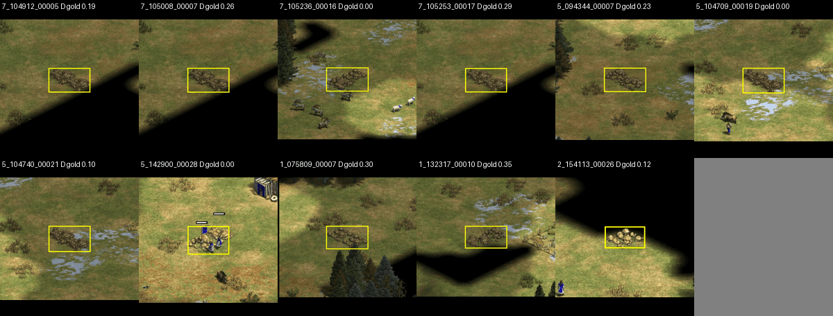
On the training screenshots, D detects 92% of the gold mines and E only 56%. D fits its training data much more closely than E, which pointed to the training process rather than the data.
Round 3: separating the optimizer from the data
Every run so far used optimizer: auto. The training logs show which optimizer it selected:
E:  optimizer: AdamW(lr=0.000145, momentum=0.9)
D:  optimizer: MuSGD(lr=0.01, momentum=0.9)
Simplified from Ultralytics 8.4.54:
iterations = math.ceil(len(train_set) / max(batch, 64)) * epochs
if optimizer == "auto":
    if iterations > 10_000:
        name, lr0 = "MuSGD", 0.01
    else:
        name, lr0 = "AdamW", round(0.002 * 5 / (4 + num_classes), 6)  # 0.000145 for 65 classes
E has 3,456 images per epoch: 54 × 150 = 8,100 iterations, so AdamW. D has 4,456: 70 × 150 = 10,500, so MuSGD with a 70× higher learning rate. The limit is at ~4,225 images. D was the only run that crossed it. Every other run in this post, including all of Round 1, trained with AdamW at 0.000145.
As a result, the comparison between D and E changed two variables at once. All runs also used seed 0, so the run-to-run variance was unknown.
To separate them, I set the optimizer explicitly and ran a 2×2: two datasets (E, D) × two optimizers, each trained twice with different seeds. Everything else stayed the same:
| Setting | AdamW runs | MuSGD runs |
|---|---|---|
optimizer | AdamW | MuSGD |
lr0 | 0.000145 | 0.01 |
momentum | 0.9 | 0.9 |
warmup_bias_lr | 0.0 | 0.0 |
seed | 0 and 1 | 0 and 1 |
warmup_bias_lr=0.0 matches what auto sets, so the new runs reproduce the earlier ones exactly. Two of the eight runs already existed (E and D), so this round was 6 new runs on three pods, ~20 GPU hours.
Test-set F1
Gold mine recall
Show the data
| Run | F1 | Gold mine recall |
|---|---|---|
| E, AdamW, seed 0 | 0.846 | 0.789 |
| E, AdamW, seed 1 | 0.834 | 0.704 |
| E, MuSGD, seed 0 | 0.860 | 0.746 |
| E, MuSGD, seed 1 | 0.862 | 0.732 |
| D, AdamW, seed 0 | 0.863 | 0.746 |
| D, AdamW, seed 1 | 0.856 | 0.676 |
| D, MuSGD, seed 0 (run D) | 0.867 | 0.648 |
| D, MuSGD, seed 1 | 0.870 | 0.732 |
| Change (both seeds pooled) | F1 | p |
|---|---|---|
| MuSGD instead of AdamW, on E data | +0.021 | 0.014 |
| MuSGD instead of AdamW, on D data | +0.009 | 0.066 |
| Adding composites, with AdamW | +0.020 | 0.002 |
| Adding composites, with MuSGD | +0.008 | 0.30 |
With AdamW at this learning rate, the model is undertrained. Switching to MuSGD and adding composites each improve F1 by about 0.02; combined, they add little more, which suggests that both address the same limitation. All Round 1 runs used AdamW, so Round 1 compared the synthetic datasets on an undertrained model.
The gold mine drop was within run-to-run variance. With seed 1, run D detects 73% of gold mines, the same as E with MuSGD. Overall F1 varies by about 0.005 between seeds, but gold mine recall varied by up to 0.085. The 71 gold mine boxes come from about 7 physical mines seen in consecutive screenshots, so a few mines determine the score. The earlier significance test compared two single runs and therefore did not account for training variance.
D also has more images, so at the same batch size it gets 29% more training steps (279 per epoch against 216). Part of the composite gain may therefore come from the additional steps.
The configuration I train with now
All settings are now explicit:
from ultralytics import YOLO

model = YOLO("yolo26n.pt")
model.train(
    data="dataset.yaml",          # real ×4 + 2,400 old synthetic + 1,000 composites
    imgsz=1280, epochs=150, batch=16,
    optimizer="MuSGD", lr0=0.01, momentum=0.9, warmup_bias_lr=0.0,
    seed=0, deterministic=True,
    patience=0,                   # no early stopping; keep the final epoch
    mosaic=1.0, close_mosaic=10, scale=0.5, translate=0.1, degrees=10,
    fliplr=0.5, flipud=0.0, mixup=0.1,
    hsv_h=0.015, hsv_s=0.7, hsv_v=0.4,
    cache="ram", workers=12,      # check the pod's RAM limit, not the GPU
)
Results are compared over at least two seeds.
The outcome
The model the agent runs now is run D. The second seed scored 0.003 higher, inside the noise, so I kept the run that had already passed the release checks. I also exported it differently: a 736×1280 input instead of 1280×1280, which fits a wide screenshot with less grey padding, and YOLO26's second output head with a separate duplicate-removal step (NMS). With the same weights, this export scores F1 0.873 and runs in 10 ms per image instead of 15 ms on an Apple M2 Pro.
Against the model the agent used before, on the same 40 screenshots:
| Model | Precision | Recall | F1 |
|---|---|---|---|
| Previous model | 0.963 | 0.748 | 0.842 |
| New model | 0.930 | 0.823 | 0.873 |
The F1 improvement is +0.031 (p = 0.045), and the new model is better in 8 of the 10 test sessions. Per class:
Show the data
| Class | Previous | New |
|---|---|---|
| villager | 0.66 | 0.80 |
| sheep | 0.45 | 0.59 |
| deer | 0.21 | 0.58 |
| boar | 0.58 | 0.96 |
| tree | 0.92 | 0.88 |
| gold mine | 0.82 | 0.76 |
It detects more animals and villagers, slightly fewer trees and mines, and produces more false detections: 77 against 36. The model is on Hugging Face as martondobos/aoe2-entity-detector.
What I'd do differently
Set the optimizer, learning rate and seed explicitly from the first run, and check the optimizer line in the training log. auto depends on the dataset size, so any experiment that changes the data can also change the optimizer. In this project the switch happened at ~4,225 images.
Keep the number of training steps equal across data experiments, or at least report it with the results.
Train every configuration at least twice. Overall F1 varied by 0.005 between seeds, while a single class varied by 0.085. A second seed would have settled the gold mine question immediately.
Measure the synthetic data before training on it. The size check took ten minutes, and the problem was not visible in the training curves.
Tools and references
- Ultralytics YOLO
Ultralytics 8.4.54: YOLO26 training, augmentation and ONNX export
- RunPod
RTX 4090 pods, one training run per pod
- X-AnyLabeling
Label review for the real screenshots and the test set
- CVAT
Label review for the real screenshots and the test set
- Hugging Face Hub (aoe2-entity-detector)
The released model, evaluation report and inference contract
- Burdorf et al., 2022
Mixing vs pretraining with synthetic data, five seeds on YOLOv3